Udacity Data Science Nanodegree Capstone Project

As part of Portfolio theory, the goal of a risk manager is to select the optimal return for the associated risk on the investment. The bank provides loan applicants with the funds required for an especific purpose and in return it gets the interest on the money lent.[0]

A correct measurement of risk allows the bank to maximize its returns with an expected level of delinquency on its loans the goal of our model is to predict as accurate as possible this suggested level of delinquency in the next two years.

In addition to the target feature analysis, we provide expected signs for our feature space as well as visualizations for each feature in Annex(A).CreditDefaultEDA

The results from our EDA analysis are summarized on this table. All of this results come from a main question: What worries me about this feature?

The logic behind expected signs is as follows. Users in financial distress tend to start using their available resources to cover the leak in their financial distress. A high utilization at high rates suggest a troublesome set.For example, A low level of liquidity, low financial knowledge sophistication ( Highest borrowing rates in the market) or non expected financial windfall, among others.

As Warren buffet once said: “ You cannot go through life borrowing at those rates” [1]

The logic behind age comes from dynamic Macroeconomic theory and the financial lifecycle. We expect (segregated by income) a Solow’s type of income stock (Savings) were the bulk of the individual’s life expenditure diminishes as life progresses,and income grows until it becomes static at retirement. [2]

Debt to income ratios suggest how much the incurred loans from the client are a burden to its day to day life, accurate income measuring its a problem in itself but when a client report 0 income to the bank, it is in the bank’s best interest to offer reestructuring facilities to weather the crisis to a client. [3]

In practice however, a low debt to income ratio paradoxically has been reported to be associated to a decrease in payment rates as well. Small amounts of debt seem to easily escape the to-do list of high income segments of population.

Regarding Past-due Events our logic relies on Merton’s modelling for financial assets. The closest you have been to default should weight on how likely you are to default in the future. Or, the standard deviation from expected returns should be priced proportionally to the expected return. A simple but elegant solution to asset pricing. [4]

This type of analysis are not possible on high dimensional feature spaces but from time to time, this low dimentional feature spaces give way for some leniency on the effect of theory on the expected results from our model.

Data Preprocessing

As part of our preprocessing techniques we will:

• Windsorize outliers according to bins defined by IQR
• Encode Missing Values

Null treatment

Identify clear Nan Values, replace with median. Median preferred due to robustness on data, and feasible value. The current state of missing values on the training set is displayed in the table below:

Outlier treatment

As part of outlier treatment of variables we will clip outliers according to the interquartile range of the population

• RevolvingUtilizationOfUnsecuredLines: [0, 0.023, 0.154, 0.559, 1.352, 2.146, inf]
• Age: [0, 18, 20, 41, 52, 63, 80, 93, float(‘Inf’)]
• NumberOfTime30–59DaysPastDueNotWorse: [0, 0.99, 1, 2, 4, 6, 10, 13, float(‘Inf’)]
• DebtRatio: [-inf, -1.904, -0.864, 0.175, 0.366, 0.868, 1.908, 2.947, inf]
• MonthlyIncome: [float(‘-Inf’), 0, 3400, 5400, 8000, 10000, 15000, 20000, 23000, float(‘Inf’)]
• NumberOfOpenCreditLinesAndLoans: [float(‘-inf’), 0, 5, 8, 11, 20, 29, float(‘inf’)]
• NumberOfTimes90DaysLate: [float(‘-inf’), 0, 1, 2, 3, 8, 10, float(‘inf’)]
• NumberOfTime60–89DaysPastDueNotWorse: bins = [float(‘-inf’), 0, 1, 2, 3, float(‘inf’)]

After preprocessing the integrity of the information holds. No records were omitted during the cleaning process, just adjusting outliers to max values inside each feature distribution.

The first approach towards model creation will be with a random Forest Classifier with the standard parameters assigned by scikit-learn.A Train/Test split at 70% of the population is defined to avoid overfitting. The model should optimize for classification metrics such as AUC, or the components of the F1-Score.

Before training our models, a quick memory sanity check is in order. The split for the training set consumes 8MB, and the Test split 3.43MB. Given the order of complexity of the models to be used, no memory shortage realted problems should arise.

Now, regarding the model, we will train a industry scikit-learn standard parameters model. More information available at https://scikit-learn.org/stable/modules/generated/sklearn.ensemble.RandomForestClassifier.html

RandomForestClassifier(random_state=42)

• bootstrap’: True
• ccp_alpha’: 0.0
• class_weight’: None
• criterion’: ‘gini’
• max_depth’: None
• max_features’: ‘auto’
• max_leaf_nodes’: None
• max_samples’: None
• min_impurity_decrease’: 0.0
• min_impurity_split’: None
• min_samples_leaf’: 1
• min_samples_split’: 2
• min_weight_fraction_leaf’: 0.0
• n_estimators’: 100
• n_jobs’: None
• oob_score’: False
• random_state’: 42
• verbose’: 0
• warm_start’: False

A pipeline object is defined in case further preprocessing techniques should arise in the future. The reported AUC score regarding this model is 0.8405 the confusion matrix is displayed below

Refinement

We implement GridSearch cross validation as implemented on Sklearn.model_selection, the chosen grid of hyperparameters are defined as follows:

• n_estimators: [20, 30, 50]
• max_depth: [2, 4]
• min_samples_leaf’: [2, 4] The best parameter combination after validation is Depth of 4, n_estimators of 20 and min_sample_lead of 4

Even a small change upon the standard chosen hyperparameters help in the classification metrics as it can be seen on the ROC plot below.

Model Evaluation and Validation¶

The model parameters are not the main objective of this article, nonetheless, the model displays a precision of 0.94 across the test set, with areas under the receiving operator curve of 0.85.

The relatively low f1 score relies entirely on the use-case. If this model is used entirely for accepting/rejecting loans, extreme care should be taken of not excluding a large percentage of the candidate population.

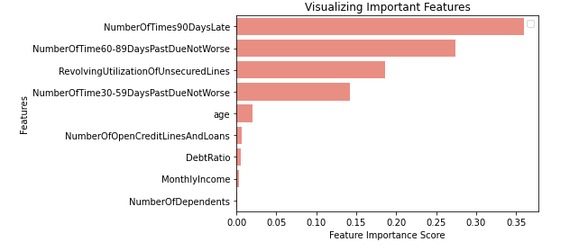
A common approach at explaining the results of a non-linear model, relies on plotting the Variable Importance for the whole population we will follow but also expand on the caveats of this approach.

Altough variable Importance shows us an important insight, regulators require granularity regarding client offerings/refusals. In order to comply to the most strict regulations we need to be able to provide reason codes for each client refused by the bank. Lets take the worst top 5predicted probabilities on our test set.

We will implement an MLI technique known as LIME ( Local Interpretable Model-agnostic Explanations ) well explained in the paper “Why Should I Trust You?”: Explaining the Predictions of Any Classifier” by Ribiero, T., et al.

This technique allows to linearize the space of joint probabilities to separate the effects of each variable on the conditional probability. In other words, assign weights of the contribution of each feature on the result of the output.

The results for the worst 4 users are displayed as follows: