Now that you have a good sense of the big picture and where logistic regression fits in the bigger scheme of things and you have an appreciation of the problem we are trying to solve, let’s get into some details.
The Classification Task
The challenge we have, now, is to provide an early warning to patients before their condition deteriorates by combining two pieces of information: heart rate and breathing rate. We would like to combine these two measurements in the best way possible to determine if a patient’s condition is deteriorating. For simplicity, we will call these situations as “abnormal”. (in the original paper, they were termed as “prodromal”). The periods when a patient’s condition is stable and there is no risk of deterioration will be called normal. The problem we have now, thus, reduces to finding out if a patient is normal or abnormal based on two measurements: Heart Rate (HR) and Breathing Rate (BR).
Classification Objective: Identify if a patient is normal or abnormal using their heart rate and breathing rate.
The Rationale for Using Multiple Features
The first question to ask is: Why do we even need two different measurements? Can’t we just use either the BR and HR and make a decision? Why complicate our lives with using multiple measurements? If you have a situation where a single measurement leads to perfect separation between normal and abnormal, you don’t need the second measurement. Graphically, this would look like this:
In fact, you don’t even need any Machine Learning for this. You can just plot the data and visually see that a simple rule that can separate the two cases would work. This simple rule, in the case of a single measurement, would graphically be a vertical line. In the figure above, this would correspond to a HR of 78. If a patient’s HR is above 78, the patient will be considered abnormal and if a patient’s HR is below 78, the patient will be considered normal. This vertical line that you see in the figure is called a “decision boundary”. For the case when you have a single measurement and such a clear separation, any vertical line that can perfectly separate the two would work (a decision boundary at 77, 78 or 79 would all be equally perfect). However, real-world problems are hard (and are problems) because such separation is not straightforward and there is a lot of overlap. Because the overlap is a lot for a single measure, we, therefore, take different types of measurement for the same patient that, although, have a lot of overlap, we hope that there is independent information coming from each measurement and by combining different measurements, we hope to find a better decision boundary that can lead to fewer errors as opposed to using only a single measurement. As an example, check the overlap present in breathing rate, heart rate and oxygen saturation in the case study (this data is available in my github repository if anyone is interested in using it. It is simulated using the same distribution of data as can be seen in the original paper referenced earlier in this post).
To keep things simple, we will use another simulated dataset, inspired by the same problem but one which shows more separation between normal and abnormal (and using only heart rate and breathing rate as stated earlier). Let us start by plotting the distribution of heart rate and breathing rate separately for both cases.
Data Visualization
As you can see, there is overlap and a single threshold for either HR or BR would lead to considerable errors. Let us plot HR and BR in a single plot so that you can visualize the problem.
The Linear Equation
If we were to combine HR and BR together to help us find the “optimal” decision boundary, what would be the simplest thing we could do? The simplest thing would be to linearly combine both the breathing rate and the heart rate. Mathematically, it would be the equivalent of finding a weighted sum, as shown in the equation below:
Graphically, this would be equivalent to finding a straight line on the 2-dimensional plot. The problem thus reduces to that of finding the correct values of A and B that can fit a line (a decision boundary) that can help us separate normal from abnormal cases.
Just a little caveat: If we only have to reduce this problem to finding A and B, then the resulting line will always pass through the origin. To remove this restriction, we can add a “bias” term and therefore, the resulting equation then becomes the following:
Thus the classification problem can conceptually be seen as finding the unknown parameters of an equation of a line that can best separate the normal and abnormal cases.
The Logistic Function
We still need to sort a few things including finding out how could we find a way to find that best line (it may look obvious at the moment for a 2-D case but remember, this is a simpler problem to help with visualization, and once we understand this, the same principle will apply to higher dimensional problems and we therefore need to find an automated and principled way of finding this).
As you can appreciate, the output of the linear combination of heart rate and breathing rate has no restriction. It can take on any value, entirely dependent on whatever the values of HR and BR could possibly be.
Wouldn’t it be convenient if the output of the equation could be converted into a probability?
It turns out there is a way to force the output of the linear combination of heart rate and breathing rate to be bounded between 0 and 1 (which can then be interpreted as a probability). To achieve this goal, all we have to do is take the output of the linear combination as an input to a new function which can take any value from -infinity to +infinity as input and then output a value between 0 and 1. One function that does this, and is used in “logistic” regression is the “logistic” function (this function is also called the sigmoid function).
You can think of this procedure as making a package of linear combination of features and then giving that package to the logistic function which will convert the output to vary between 0 and 1. However, this conversion is not random. If you look closely at the logistic function, you will notice that it outputs a value >0.5 for any positive input and a value of <0.5 for any negative input. So all we need to do is find the values of A, B, C (from the equation defined earlier) such that the linear equation outputs a very large negative value for cases where the real value is 0 (to follow convention, we assign 0 to normal cases), and it outputs a very large positive value when the real value is 1 (1 correspond to cases where the patient is abnormal). Or to rephrase this in simpler words: we need to find the values of A,B,C such that the output of the logistic function is close to the actual value.
The Cost Function
One way to do this would be to define a “cost” function. And this cost function needs to ensure that it outputs a large value when the output from the logistic function is very different than the actual value (say the real value is 1 and the logistic function is outputting a very small value, close to 0 or if the real value is 0 and the logistic function is outputting a large value close to 1). Conversely, this cost function needs to output a very small value and ideally 0 when the output matches the actual value. If we can have such a cost function, then all we have to do is find the values of parameters A,B,C that results in the smallest (the minimum) cost function.
The Optimization
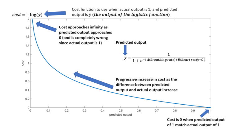
The procedure of finding the minimum value of cost function is called “optimization”. How are we going to do this? We can use calculus (more specifically, a gradient descent algorithm which helps us find the minimum of a function). While, in theory, we could use several mathematical functions that can have this characteristic (high cost value when difference is high, and low cost value when difference is low), we also need to make sure that the function is “convex”. This then helps us use calculus to easily find the value of parameters where the cost is a minimum. If we don’t have a convex function, then we may not necessarily find a global minimum and it will not be an optimal solution. Thankfully, the requirement of cost function for logistic regression has already been well researched and worked out and graphically, it looks like the following when the actual output is 1. To reinforce the concepts, I have labelled the figure. The cost function is dependent on the predicted value and from the figure, we can see that the cost is 0 when there is a complete match between the actual output and the predicted output, and the cost progressively increases as the difference between predicted and actual value increase.
If you have grasped the cost function figure above, then the next one should be immediately clear (which is a mirror image of the earlier figure and depicts the scenario when the actual output is 0).
Once you have the cost function defined, all you need to do now is run an optimization algorithm and find the value of the unknowns that can help get you the minimum. To start the optimization process, we need to initialize the values of the unknowns to some values. Subsequently, we can then run the function and get the values of the unknown parameters for which the cost function is a minimum. Having run this, in our problem, we get the following decision boundary.
The Prediction
Finally, if we need to make prediction on a new dataset, all we need to do is get their HR and BR, and use the parameter values found (A,B, and C) during learning to find out the predicted output, y. Graphically, this would be equivalent to determining which side of the decision boundary the new data point lies in. If it is above the line, the patient can be considered normal. If it is below the line, the patient can be considered abnormal.
Implementation from Scratch
To keep the post brief, I will share the key points of how to implement logistic regression from scratch. However, you can check my github repository to access the code that produced the figures in this post (implemented in Matlab). If there is interest, I will subsequently also share Python and R code in the repository as well. The key implementation steps are:
(i) Get the data in a matrix form
(ii) Visualize data (scatter plot to see correlations, histograms or density plots to get a better sense of the distribution of data)
(iii) Add the intercept (the bias) term
(iv) Initialize the unknown parameters (any random numbers would work in this case)
(v) Define the cost function and run the optimization routine (you will find built-in routines in any programming language of your choice to do that)
(vi) Plot the decision boundary
(vii) Make predictions
The various equations that need to be implemented have been given in the post here (see the two cost function graphs). It should be simple to follow this article in combination with the code to help you figure out the complete pipeline and implement it yourself.