Chi Square Test for Independence of Attributes
Consider the following questions:
1. Is their any association between income level and brand preference?
2. Is their any association between family size and size of washing machine bought?
3. Are the attributes educational background and type of job chosen independent?
The solutions to the above questions need the help of Chi-Square test of independence in a contingency table. Please note that the variables involved in Chi-Square analysis are nominally scaled. Nominal data are also known by two names — categorical data and attribute data.
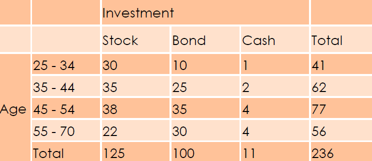
Contingency Table: Is there any relation be-tween age and investment?
Assumptions
1. The data should be categorical variables
2. Total frequency should be reasonably large, say greater than 50
3. The observations of the sample are independent, i.e., the samples are random
4. The theoretical frequency of any category or class should not be less than
Hypotheses of the test are
H0: There is no association between the variables
H1: There is an association between the variables
Calculation of Chi Square Statistic
Calculation of Theoretical Frequency
Remember, Chi square test of independence only checks whether there is any association between the attributes, but it does not tell what is the nature of the association.
Correlation Analysis
The simplest way to look at whether two variables are associated is to look at whether they covary. To understand what covariance is, we first need to think back to the concept of variance.
Variance = Σ (xi — mx)2 / (N — 1) = Σ (xi — mx) (xi — mx)/ (N — 1)
The mean of the sample is represented by mx, xi is the data point in question and N is the number of observations. If we are interested in whether two variables are related, then we are interested in whether changes in one variable are met with similar changes in the other variable.
When there are two variables, rather than squaring each difference, we can multiply the difference for one variable by the corresponding difference for the second variable. As with the variance, if we want an average value of the combined differences for the two variables, we must divide by the number of observations (we actually divide by N — 1). This averaged sum of combined differences is known as the covariance:
Cov(x,y) = Σ (xi — mx) (yi — my)/ (N — 1)
There is, however, one problem with covariance as a measure of the relationship be-tween variables and that is that it depends upon the scales of measurement used. So, covariance is not a standardized measure. To overcome the problem of dependence on the measurement scale, we need to convert the covariance into a standard set of units. This process is known as standardization. Therefore, we need a unit of measurement into which any scale of measurement can be con-verted. The unit of measurement we use is the standard deviation.
The standardized covariance is known as a cor-relation coefficient.
r = covxy / sx sy = Σ (xi — mx) (yi — my)/ [(N — 1) sx sy] which always lies in between –1 and 1. Remember, correlation doesn‘t necessarily imply causation.
Test of Hypotheses for Correlation
For pairs from an uncorrelated bivariate normal distribution, the sampling distribution of Pearson’s correlation coefficient follows Student’s t-distribution with degrees of freedom n − 2. Specifically, if the underlying variables have a bivariate normal distribution, the variable
has a Student’s t-distribution in the null case (zero correlation).
Partial Correlation
A correlation between two variables in which the effects of other variables are held constant is known as partial correlation. The partial correlation for 1 and 2 with control-ling variable 3 is given by:
r12.3 = (r12 — r13 r23) / [√ (1 — r132) √ (1 — r232)]
For example, we might find the ordinary correlation between blood pressure and blood cholesterol might be a high, strong positive correlation. We could potentially find a very small partial correlation between these two variables, after we have taken into account the age of the subject. If this were the case, this might suggest that both variables are related to age, and the observed correlation is only due to their com-mon relationship to age.
