Using Machine Learning to Predict NBA Team Wins

While some maverick sports veterans like Charles Barkley view analytics as “crap,” others among the newer, big-data school of thought, view statistics as a vital aspect of professional sports altogether (like Billy Bean and the Oakland A’s in the early 2000s).

But, who is more correct?

Is it a player’s feel for and experience with their sport that makes them win more than their opponents? Or, can we abstract their game to figures and stat-lines to predict future performance?

As a beginner statistician, I lie firmly on the Moneyball side of the argument. My ultimate goal is to prove the Charles Barkley’s of the world wrong and to demonstrate that large numbers can accurately predict a team’s or a player’s performance.

In this project, I hope to demonstrate this idea with entire NBA teams as my subjects. I will gather time-series data over decades regarding each team’s offensive and defensive production. I will then construct machine learning models to predict those NBA teams’ win counts at the end of any inputted season.

As we have only just passed the 1/3 mark of the 2020–21 season, this article’s predictions may prove intriguing come play-in series time (which are set for May). As such, I will re-run my models throughout the season and provide updates to my predictions in subsequent articles.

As this is the beginning of my documented data science learning journey, I wanted to ensure that any data collection frameworks I created would be generalizable and relatively future-proof. This requirement was important to me because I wanted the ability to re-evaluate my projects in the future as I improve.

In the scope of this project, this meant creating a collection script that would be easy-to-use and that would work for future NBA seasons.

Before I talk about my data scraping framework, I’ll first discuss the data which I used to power this project.

In short, it all comes from the amazing basketball-reference.com.

Basketball-Reference is my go-to site for NBA stats. In addition to succinctly organizing information on each player and team, Basketball-Reference features a relatively simple backend HTML structure. This simpler HTML proved incredibly useful as my web-scraping script relied on BeautifulSoup to somewhat manually traverse it.

After a brief exploration of Basketball-Reference for data that would operate well in my model, I stumbled upon what I consider to be the perfect webpage for this project. This ended up being the season summary pages. Linked here, Basketball-Reference season summary pages provide ample data on how each team performed both offensively and defensively in a given season. This page also contains potentially useful data like whether a certain team makes the playoffs, how many wins they had, and so much more.

This singular webpage contained so much useful data for this project that I ended up gathering from it 51 potentially relevant independent variables for my models (which I will likely need to trim down).

This deep dive into web scraping with Python proved both tedious and incredibly useful as a learning opportunity. For any inexperienced data scientists like myself starting out on independent projects, I recommend working on ones that implement web scraping in some way. Using packages like BeautifulSoup is useful not only constructive for learning the in’s and out’s of grabbing data from external sources, but also serves as an excellent opportunity to gain an understanding of how webpages are structured through HTML, CSS, and javascript in the backend.

One of the many challenges in scraping NBA team data was that Basketball-Reference stowed away the data I was looking for into HTML comment blocks. I won’t go very deeply into the challenges like these that I encountered for fear of putting my readers to sleep. However, I’ve documented these challenges more thoroughly as comments on my actual script, ScrapeNBATeamData.py (linked here and below).

tl;dr
The result of my efforts is a generalizable script that given a range of two years between 1970 and the modern-day, returns a Pandas dataframe of cleaned team stats.

If you would like to use my NBATeamDataScraper, here is the link to my relevant GitHub page.
If you use my script, make sure to credit me in some way in your project!

Now, for the fun part!

After my data scraping was complete, I transitioned into a Jupyter Notebook to begin the initial data analysis and model-building portion of this project.

In this first go-at-it, my main objective was to simply give this project some legs. That said, my initial data analysis is less detailed than that of a seasoned data scientist. However, with subsequent articles and more learning on my part, that side of my writing will expand.

In order to get this project off the ground with a functional model, some initial data remodeling was necessary though.

Two paragraphs below this point is a screenshot of all 51 X-variables that I scraped from basketball-reference. ‘_OPP’ at the end of the variable implies that it refers to how a given team’s opponent performs in that category. For example, if you are the home team, ORB represents how many offensive rebounds your team grabbed per game. ORB_OPP by contrast tells us how many offensive rebounds the opponent team grabbed per game.

Incorporating opponent data allows us to gauge the effectiveness of a subject team’s defense. Because, of course, a better defense for the said subject team would imply that their opponents score fewer points, make baskets at a lower efficiency, etc, etc.

51 independent variables make for quite a ton of data. And, upon first glance, some of you may see certain variables that may by their very nature confound a potential ML model. If you don’t a clue what these potential problematic variables may be though then no need to fear; I will explain what each is below.

Confounding variables:

Wins: As the goal of our project is to predict the number of wins that a team ends up with, it wouldn’t make sense to keep this as an independent variable in our model.

PLYF: This variable refers to whether a team makes the playoffs or not. Including this would likely overfit our model and overshadow other variables in their relative importance to # of wins.

Rnk: Rnk refers to the team’s rank in their respective Eastern or Western conference (each conference has 15 teams). This one is also a no-brainer to drop as a team’s rank is excessively correlated with their number of wins.

Team: Team is a variable that refers to a franchise’s name (like the Boston Celtics). Including this variable may account for certain less-measurable factors that make a team great, like coaching, scouting, and organizational management. However, I ultimately decided to remove it from the model for two reasons. For one, a team’s performance can change in the blink of an eye with the hiring of a new coach or GM. And two, it may severely overrate certain teams who have been incredibly successful over many years (like the San Antonio Spurs).

Dropping potentially confounding variables was not the only necessary pre-processing step to generate an initial model. Next, I made sure that my variables were normalized with respect to one another.

Normalization is the process of bringing values in one’s data set into a common scale, usually either from -1 to 1, or 0 to 1. In my case, it ensures that any model that I create for this project doesn’t overrate variables like two-pointers attempted (whose value is generally around 45–55) compared to two-pointer percentage (which is measured as a value somewhere between 0.00–0.60) simply because their range of values are so different.

Here is a link to an informative (and free) video to better understand normalization provided by Coursera. Thanks, Coursera!

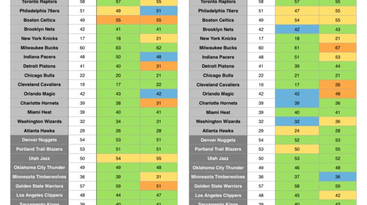
After I normalized my variables, I could finally move on to model construction. I implemented a simple linear regression, as well as a more complex neural network.

I tested the precision of both by comparing their predictions of the 2018–19 NBA regular season versus the actual number of wins per team. I did not opt for 2020 as the target year as the number of wins per team was heavily influenced based on whether said team participated in the NBA bubble. I also chose to test the effectiveness of either model with both 2000–2018 and 2010–2018 as ranges of training data. Comparing the results of the 2000–2018 and 2010–2018 model with the actual results of the 2021 season may give us extra insight into whether the way professional basketball is played truly has changed in the past decade (with an emphasis on three-pointers and high-percentage 2’s).

Just how accurate is our model???

Drumroll, please!

But wait! Before we do that, what would we consider success for our models?

Well, the average number of wins for teams in the NBA’s 82 game regular season is 42 (exactly half). As such, an accurate model to us would be one with an average win count as close to 42 as possible. But, there could be a model that is close to a 42 average that is filled with an equal amount of predictions +7 or -7 wins from their target. Of course, that would not be an acceptable outcome.

So, a successful model would be also be defined as one where the difference between the actual and predicted win values has a relatively low range for all teams.

With those criteria in mind, below are the model’s predictions for each team in the 2019 NBA regular season.

Eastern Conference teams are listed in light gray, WC teams are in dark gray: