An introduction to Bayesian approximations for Neural Networks
Bayesian analysis is a great way to quantify the uncertainty of a model’s predictions.
Most regular machine learning modelling tasks involve defining a likelihood function for data given a model and its parameters. The aim is to maximise that likelihood with respect to the parameters in a process known as Maximum Likelihood Estimation (MLE). MLEs are point estimates of the model parameters, this means a single prediction is made MLE parameters are used in inference.
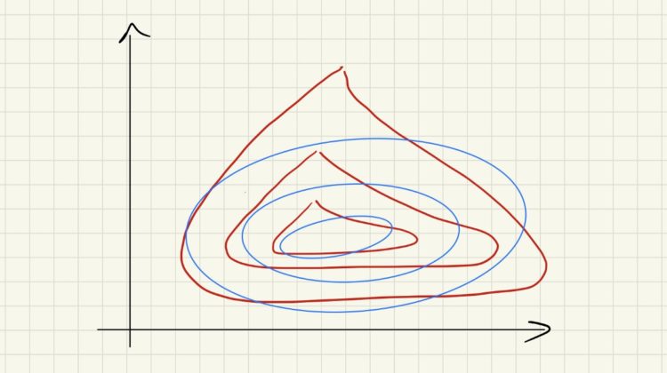
In Bayesian modelling, in addition to the likelihood function, we must also define prior distributions for the model parameters. We use Bayes’ rule to find the posterior parameter distribution. The posterior distribution and model can be used to produce a probability distribution of the prediction (shown below). This is what allows us to quantify uncertainty when using Bayesian modelling methods. If we’re no longer bound to point estimates, we can choose whether or not to trust the model’s prediction based on the spread of the distribution.
That’s all very well but what’s the catch? Bayesian inference is often a very expensive endeavour. Calculating the posterior distribution is often either intractable or extremely analytically difficult. Furthermore, even if there is a closed analytical form for the posterior, calculating the integral over all parameters is basically impossible for models of any reasonable complexity.
There are ways to mitigate this difficulty:
- Maximum Aposterior Estimate (MAP) finds the peak of the posterior distribution and use this as a point estimate for the model (this is often better than using just the likelihood but doesn’t give us a measure of uncertainty for our predictions).
- Markov Chain Monte Carlo (MCMC) which allows us to draw samples from the posterior. However, it can be extremely slow, especially for large models and datasets and it doesn’t work well with highly multimodal posterior distributions.
- Variational Inference (VI) approximates the posterior with a simpler, “well behaved” distribution. This is what we’re going to explore for the rest of this article.
What is Variation Inference (VI)?
Variational Inference aims to approximate the posterior with a “well behaved” distribution. This means that integrals are computed such that the better the estimate, the more accurate the approximate inference will be. Let’s take a look at some maths and then we’ll see how this applies to neural networks.
First, we need to define a distance measure between probability distributions that we can use to minimise. For this, we choose a distance measure called the Kullback-Liebler (KL) divergence. The reason we choose the KL divergence over other distance measures will become clear in a moment but it’s basically because of it’s close ties to the log-likelihood.
KL has the following form:
If we substitute the p(x) term for the posterior and do a bit of rearranging we get…
Now we can use the fact that the KL divergence is always positive in the following way…
The F(D,q) term is called the variational free energy or the Evidence Lower Bound (ELBo). Importantly, maximising the ELBo minimises the KL divergence between the approximate posterior and the true posterior. The form of the free energy in the last line is the form that’s most useful to us for the purpose of optimization.
We brushed over a detail before, I said we need to approximate the posterior with a “well behaved” distribution but what constitutes “well behaved”? One popular choice is to approximate the joint posterior of all parameters as the product of independent distributions (often Gaussians). The independence condition allows for a number of optimisation methods to be used to maximise the ELBo including coordinate ascent and gradient ascent. Gaussians are chosen for a number of reasons including the fact that they are a conjugate prior and the KL between Gaussians has a clean closed-form.
How does this apply to Neural networks?
So how can we apply VI and the mean-field approximation to neural networks?
The transition from a non-Bayesian to a variational-Bayesian network is quite a smooth one. Normally we would create a dense layer with weights in it but these are just point estimates, now we want to model each weight as an approximate posterior distribution. So let’s say each weight has a Gaussian posterior with mean μ and standard deviation σ.
To maximise the ELBo we need two things, the mean likelihood over the approximate posterior (q) and the KL between q and the prior. To compute the mean likelihood we draw Monte Carlo samples from q and estimate the mean likelihood by taking a forward pass of a minibatch (like we would do normally). The KL between q and the prior has a nice closed form because we chose everything to be Gaussian.
Then we can use just use gradient descent as normal right? Well not quite, there is a small subtlety, you can’t take gradients of something stochastic, it just doesn’t make sense. So here’s another reason to choose a Gaussian, you can parameterise a Gaussian in the following way:
Now we can take gradients with respect to μ and σ!
It’s worth noting that we’ve not doubled the number of parameters in our model since we now have a separate weight for the mean and standard deviation of each model parameter. This increases the complexity of the model quite substantially without improving the model’s predictive power.
What does that look like in PyTorch?
Well, it looks like this…
There are a few important things to note with this implementation. Firstly, we don’t create weights for the variance directly. Instead, we create weights such that σ = log(1+exp(w)). We do this for numeric stability during optimisation. The second thing is that we accumulate the KL loss for each layer and as you’ll see in a moment, we pass that loss forward to the next layer. We can do this because the KL term doesn’t depend on the data and it helps us to keep tabs on the total KL loss if we just add it up as we go.
Now let’s put this into a model:
Lovely in theory but does it actually work?
Great question! Let’s find out! Let’s take MNIST, train a model to classify handwritten digits and see what the results look like. I haven’t included the training loop code here because it’s all pretty boilerplate, nothing fancy, just train a model on MNIST for about 5 epochs.
One thing that is worth noting is that when we use this model to make predictions, we want to predict multiple times using samples from q. That way we unleash the real power of Bayesian networks which is the ability to predict uncertainty. Knowing when your model is confident about a prediction can help us to include a human in the loop and improve our overall accuracy by only accepting predictions that the model is confident with.
To create this figure all points are ordered based on the uncertainty in the prediction. We then iteratively discard predictions based on their uncertainty and evaluate the new model accuracy. If we predict on all of the data, regardless of our certainty, we can expect a validation accuracy of about 93%. By flagging only 5% of the data we can boost model accuracy by more than 2%! In general, the higher the proportion of predictions that we flag for review, the higher the accuracy achieved by the model. We could use this method to calculate a threshold uncertainty that should be used to decide if a prediction should be flagged for review or not.
We can also take a look at some samples that the model isn’t confident about…
In this case we predicted a 3 but the label is a 5… to be honest I don’t know about you but I can see where the confusion comes from!
What have we learnt?
We’ve hopefully achieved 2 main objectives in this post. Firstly, we understand what variational inference is and why it’s useful and secondly, we know how to implement and train a deep neural network that leverages VI. So next time you’re designing a run-of-the-mill neural net for classification or regression, consider making it Bayesian instead!