Visualizing Learning of a Deep Neural Network

Using Deep Replay for Visualizing the Neural Network Learning

Deep Learning is generally considered a black box technique because you generally can’t analyze how it is working in the back-end. You create a deep neural network, compile it, and then fit it on your data, we know that it will work using neurons transferring the information using different layers and all the activations and other important hyperparameters. But we can’t visualize how information is being transferred or how the model is learning.

What if I tell you that there is a python package that creates the visualizations of how the model is working or learning at each iteration/epoch. You can use this visualization for educational purposes or presenting it to others to show them how your model is learning. If this excites you then you are at the right place.

Deep Replay an open-source python package designed to allow you to visualize a replay of how your model training process is carried out in Keras.

Let’s get started…….

For this article, we will be using google colab and in order to use this, we will first need to set up a notebook. Copy and run the code given below in order to make your notebook ready.

# To run this notebook on Google Colab, you need to run these two commands first
# to install FFMPEG (to generate animations - it may take a while to install!)
# and the actual DeepReplay package!apt-get install ffmpeg
!pip install deepreplay

This command will also install our required library i.e. deep replay.

As we are working on creating a deep neural network so we need to import the required libraries.

from keras.layers import Dense
from keras.models import Sequential
from keras.optimizers import SGD
from keras.initializers import glorot_normal, normalfrom deepreplay.callbacks import ReplayData
from deepreplay.replay import Replay
from deepreplay.plot import compose_animations, compose_plotsimport matplotlib.pyplot as plt
from IPython.display import HTML
from sklearn.datasets import make_moons%matplotlib inline

In this step, we will load the data that we will be working on and we will create a callback for a replay of the visualization.

group_name = 'moons'X, y = make_moons(n_samples=2000, random_state=27, noise=0.03)replaydata = ReplayData(X, y, filename='moons_dataset.h5', group_name=group_name)fig, ax = plt.subplots(1, 1, figsize=(5, 5))
ax.scatter(*X.transpose(), c=y, cmap=plt.cm.brg, s=5)

Now we will create the Keras model using different layers, activation, and all other hyperparameters. Also, we will print the summary of the model.

sgd = SGD(lr=0.01)glorot_initializer = glorot_normal(seed=42)
normal_initializer = normal(seed=42)model = Sequential()
model.add(Dense(input_dim=2,
units=4,
kernel_initializer=glorot_initializer,
activation='tanh'))
model.add(Dense(units=2,
kernel_initializer=glorot_initializer,
activation='tanh',
name='hidden'))model.add(Dense(units=1,
kernel_initializer=normal_initializer,
activation='sigmoid',
name='output'))model.compile(loss='binary_crossentropy',
optimizer=sgd,
metrics=['acc'])model.summary()

Let’s train the model Now

While training the model we will pass the callback to the fit command.

model.fit(X, y, epochs=200, batch_size=16, callbacks=[replaydata])

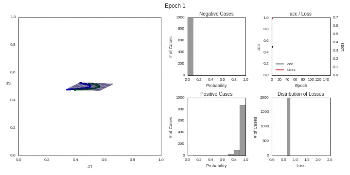
Now we will create some empty plots on which we will plot our data related to the learning of the model.

fig = plt.figure(figsize=(12, 6))
ax_fs = plt.subplot2grid((2, 4), (0, 0), colspan=2, rowspan=2)
ax_ph_neg = plt.subplot2grid((2, 4), (0, 2))
ax_ph_pos = plt.subplot2grid((2, 4), (1, 2))
ax_lm = plt.subplot2grid((2, 4), (0, 3))
ax_lh = plt.subplot2grid((2, 4), (1, 3))

In the next step, we just need to pass the data into these empty visualizations and create a video of all the iterations/epochs. The video will be containing the learning process at each epoch.

replay = Replay(replay_filename='moons_dataset.h5', group_name=group_name)fs = replay.build_feature_space(ax_fs, layer_name='hidden',
xlim=(-1, 2), ylim=(-.5, 1),
display_grid=False)
ph = replay.build_probability_histogram(ax_ph_neg, ax_ph_pos)
lh = replay.build_loss_histogram(ax_lh)
lm = replay.build_loss_and_metric(ax_lm, 'acc')

Creating a Sample Plot

sample_figure = compose_plots([fs, ph, lm, lh], 160)
sample_figure

Creating The Video

sample_anim = compose_animations([fs, ph, lm, lh])
HTML(sample_anim.to_html5_video())

This is how we can use Deep Replay for the Deep Neural Network training process.Go ahead try this and let me know your experiences in the response section.

This article is in collaboration with

.

Thanks for reading! If you want to get in touch with me, feel free to reach me on hmix13@gmail.com or my LinkedIn Profile. You can view my Github profile for different data science projects and packages tutorials. Also, feel free to explore my profile and read different articles I have written related to Data Science.