While searching for a dataset to apply machine learning techniques I came to this wine reviews dataset. The dataset consist of categorical data, text and numerical data. The data consists of 9 columns where variety is the output column where prediction is to be done. The proposed model is a cascading model which uses country, province, points, winery, price for prediction of variety.
1)Understanding the dataset
The dataset is loaded into the the variable data. The data is not clean it should be preprocessed and the null values should be filled.
data=pd.read_csv(‘data.csv’)
print(data.describe())
print(data.info())
2)Cleaning and Pre processing the data
By observing the data it can be noted that the attribute user_name has about 20000 null values. It seems to have almost no effect to predict the variety so the feature is dropped, Similarly, the price has about 5000 null values. So, the null values was imputed using the mean values.
data[‘price’].fillna(value=data[‘price’].mean(), inplace=True)
data=data.drop([‘user_name’], axis=1)
print(data.info())
Finally, all the null values are removed. Now the data can be encoded and divided into training and test split.
3)Performing Basic Exploratory Data Analysis
EDA is usually performed to understand the trend of the data. In this blog basic EDA is performed. Initially a plot showing the distribution of point vs average price of point was generated. It can be observe that as the points increase the average price also tends to increase. Also, it can be seen that the Bordeaux-style Red Blend and Bordeaux-style White Blend have the highest average price in terms of variety.
import plotly.express as px
wd_price = data.groupby(‘points’)[‘price’].mean().reset_index()
wd_price.head()
fig = px.scatter(x=wd_price[‘points’], y=wd_price[‘price’], title = ‘Price Distribution against Points’)
fig.show()
wd_variety = data.groupby(‘variety’)[‘price’].mean().reset_index()
print(“The average price of Wine per variety”)
wd_variety.head()
4)Feature Encoding and data set splitting
The variety feature that is to be predicted was separated as ‘y’ and rest of the feature as X. Also as the attribute y has categorical features the ordinal encoder was used to convert the categories into numbers such that computer can understand it. Also the dataset was divided into train test set with stratifying using y which means the distribution of y feature in train and test set is similar.
from sklearn.preprocessing import OrdinalEncoder
y = data[‘variety’].values
oe = OrdinalEncoder()
y = oe.fit_transform(y.reshape(-1,1))
X = data.drop([‘variety’], axis=1)
from sklearn.model_selection import train_test_split
X_train, X_test, y_train, y_test = train_test_split(X, y, test_size=0.33, stratify=y)
The data set has two features as text (review title and review description) which were vectorized using TF-IDF vectorizer. Also, Count Vectorizer was used on categorical features : country, winery and province , and normalizing was done the numerical feature price and points. Finally all the features were stacked together.
from sklearn.feature_extraction.text import TfidfVectorizer
vectorizer = TfidfVectorizer(min_df=10)
vectorizer.fit(X_train[‘review_title’].values)
X_train_title= vectorizer.transform(X_train[‘review_title’].values)
X_test_title= vectorizer.transform(X_test[‘review_title’].values)
vectorizer.fit(X_train[‘review_description’].values)
X_train_review= vectorizer.transform(X_train[‘review_description’].values)
X_test_review= vectorizer.transform(X_test[‘review_description’].values)
vectorizer = CountVectorizer()
vectorizer.fit(X_train['country'].values)
X_train_country = vectorizer.transform(X_train['country'].values)
X_test_country= vectorizer.transform(X_test['country'].values)
vectorizer = CountVectorizer()
vectorizer.fit(X_train['winery'].values)
X_train_winery = vectorizer.transform(X_train['winery'].values)
X_test_winery= vectorizer.transform(X_test['winery'].values)
vectorizer = CountVectorizer()
vectorizer.fit(X_train['province'].values)
X_train_province = vectorizer.transform(X_train['province'].values)
X_test_province= vectorizer.transform(X_test['province'].values)
from sklearn.preprocessing import Normalizer
normalizer = Normalizer()
normalizer.fit(X_train['price'].values.reshape(-1,1))
X_train_price = normalizer.transform( X_train['price'].values.reshape(-1,1))
X_test_price=  normalizer.transform(X_test['price'].values.reshape(-1,1))
normalizer.fit(X_train['points'].values.reshape(-1,1))
X_train_points =normalizer.transform( X_train['points'].values.reshape(-1,1))
X_test_points=normalizer.transform(X_test['points'].values.reshape(-1,1))from scipy.sparse import hstack
X_tr = hstack((X_train_country,X_train_points,X_train_price,X_train_province,X_train_review,X_train_title,X_train_winery)).tocsr()
X_te=hstack((X_test_country,X_test_points,X_test_price,X_test_province,X_test_review,X_test_title,X_test_winery)).tocsr()
5)Creating various Base learners
The base model used for the stacking classifier were KNN, Logistic Regression, Random Forest and GBDT. Also, two stacking classifiers with meta classifier as Logistic Regression and GBDT where trained and the accuracy were reported. The hypermeters of the base learners were tuned using 3 fold cross validation.
from sklearn.metrics import accuracy_score, f1_score
from sklearn.model_selection import GridSearchCV
from sklearn.neighbors import KNeighborsClassifier
tuned_parameters = [{‘n_neighbors’: [3,5,12]}]
model = GridSearchCV(KNeighborsClassifier(), tuned_parameters, scoring = ‘accuracy’, cv=3)
model.fit(X_tr, y_train)
print(model.best_estimator_)
print(“The accuracy of KNN model is: “,model.score(X_te, y_test))
from sklearn.metrics import accuracy_score, f1_score
from sklearn.model_selection import GridSearchCV
from sklearn.linear_model import LogisticRegression
from sklearn.metrics import accuracy_score, f1_score
tuned_parameters = [{'C': [10**-4, 10**-2, 10**0, 10**2]}]
model = GridSearchCV(LogisticRegression(), tuned_parameters, scoring = 'accuracy', cv=3)
model.fit(X_tr, y_train)
print(model.best_estimator_)
print("The accuracy of LogisticRegression model is: ",model.score(X_te, y_test))
from sklearn.ensemble import RandomForestClassifier
tuned_parameters = [{'max_depth':[5,10,12]}]
model = GridSearchCV(RandomForestClassifier(), tuned_parameters, scoring = 'accuracy', cv=3)
model.fit(X_tr, y_train)
print(model.best_estimator_)
print("The accuracy of LogisticRegression model is: ",model.score(X_te, y_test))
from sklearn.ensemble import GradientBoostingClassifier
grid=GradientBoostingClassifier(max_depth=5,n_estimators=70)
grid.fit(X_tr,y_train)
print(grid.score(X_te,y_test))
6)Creating Stacking classifiers
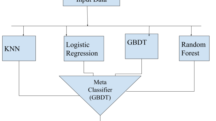
The architecture of the stacking classifier is depicted in figure 2. It uses KNN, Logistic Regression, Random Forest and GBDT as base learners and the meta classifier used was also the GBDT model. The stacking classifier were trained with the tuned hyper parameters of the base learners.
from sklearn.neighbors import KNeighborsClassifier
from sklearn.ensemble import GradientBoostingClassifier
from sklearn.ensemble import RandomForestClassifier
from sklearn.linear_model import LogisticRegression
clf1=KNeighborsClassifier(n_neighbors=3)
clf2=LogisticRegression(C=100,max_iter=5000)
clf3=RandomForestClassifier(max_depth=12)
clf4=GradientBoostingClassifier(max_depth=5,n_estimators=70)
lr=LogisticRegression(max_iter=5000)
import mlxtend
from mlxtend.classifier import StackingClassifier
sclf = StackingClassifier(classifiers=[clf1, clf2, clf3,clf4],
meta_classifier=clf4)
sclf.fit(X_tr,y_train.ravel())
print(sclf.score(X_te,y_test.ravel()))
It can be seen that some base learns perform better than the stacking classifier in terms of accuracy (logistic regression). However, the stacking classifier uses the base learners in such a way that even with models with about 70% accuracy are combined to provide accuracy of 97.3%.